gis
Overview
In this task we are provided with two DEMs for Pats Cabin Reach of Bridge Creek. One was created from raw survey data collected in 2010 and the other from a survey done in 2011. Your job is to analyze this data for potential change in the channel, then create a map clearly illustrating any areas of erosion or deposition that occurred between 2010 and 2011.
Data
The DEMs you need for the analysis can be found in the Lab07_PatsCabin_DoDInputs.zip ![]() file. You will also want to download the DoD_Classed_2.5m.lyr file, because you will use the symbology from this layer to display your DEMs. Note: you don’t need to add this layer file to your map.
file. You will also want to download the DoD_Classed_2.5m.lyr file, because you will use the symbology from this layer to display your DEMs. Note: you don’t need to add this layer file to your map.
You will also create a model that automates the process of filtering out the noise in the DEM of difference (DoD) that you create. More details below.
One way to accomplish this task:
- Create an initial DEM of difference (DoD). (Subtract one DEM from another [order matters: think about negative numbers being erosion])
- Remove the cells that contain ‘change in elevation’ values you aren’t confident in (see below for more details)
- Map areas of erosion or deposition with effective symbology
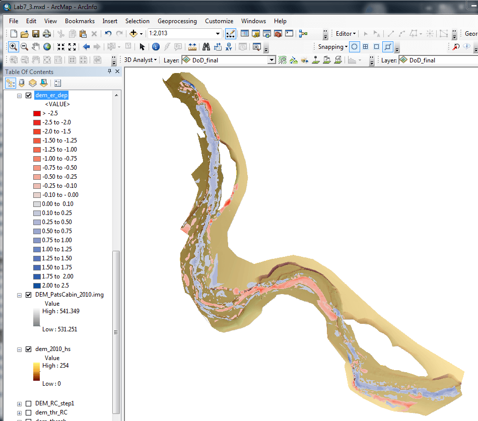
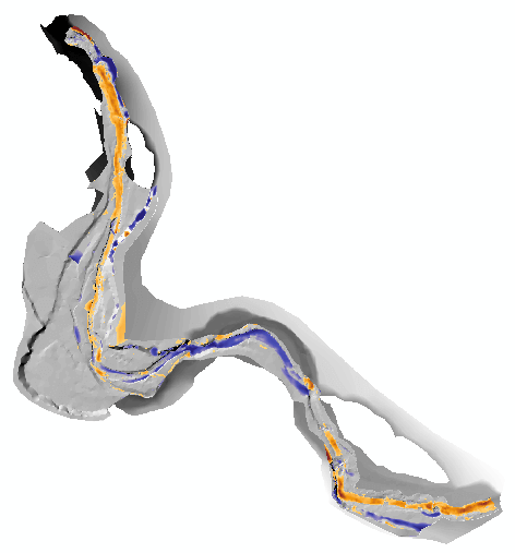
DoD (with 20 cm confidence threshold applied) displayed over DEM/Hillshade of Pats Cabin reach of Bridge Creek. Blue maps areas of deposition, red maps areas of erosion.
A little more detail:
- Download the Lab07_PatsCabin_DoDInputs.zip file. Extract all files; you will only need the DEMs from 2010 and 2011. Also download the DoD_Classed_2.5m.lyr file. You will only use this for its symbology, so you don’t need to add it to your map document.
- Create a DEM of Difference: use the raster calculator to subtract the 2010 DEM from the 2011 DEM (output is the initial DoD)
- Using a 20 cm confidence threshold (+/-10cm), run a raster calculator on the DoD to output a new raster containing the DoD cells that are greater than 10cm change and less than -10cm change (output is binary raster with values 0 and 1)
- Reclassify binary raster changing 0 (false) values to NoData (case sensitive) and true values to 1
- Multiply initial DoD by new (Reclassified) binary raster to preserve values you are confident in and remove (convert to NoData) elevation change values between -10cm and 10cm (those you are not confident in)
- Apply a stretched color ramp (red to blue diverging, bright [for example] - with blue representing areas of deposition) to your edited DoD and evaluate your results
- Now import symbology for the Dod from the Dod_classed_2.5.lyr (to improve effectiveness of symbology)
Evaluate your results considering the following information about the site: The reach has 13 beaver dams and/or support structures installed. After 2011 high flows, most of the top of reach ponds filled in completely with sediment. There was avulsion in the middle reach where significant downcut occurred as a result of the blowout of one of the major dams. The lower reach ponds aggraded substantially.
Model Building
Model building is a way to automate your work. “When you create a model, you are preserving a set of tasks, or a data processing workflow, that you can execute multiple times.” (ESRI)
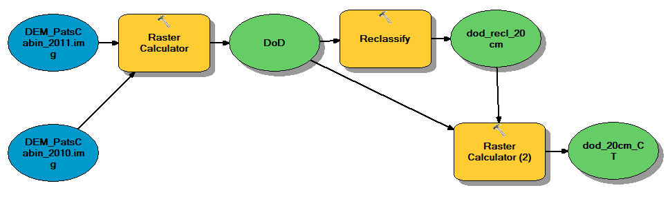
You will build a model to automate the process of creating a DoD with the 20cm confidence threshold (steps 2-5 in the “A little more detail” section above). It might be helpful to run through the process so you know how the tools and inputs function. But you can go ahead and build the model first and use it to create a DEM of difference with the applied confidence threshold, if you feel comfortable with the process.
You can use the following video tutorials to acquaint yourself with model building in ArcGIS. The tutorial uses a different work flow (watershed delineation) but the process of model building is the same and should be pretty easy to follow. Again, you might want to run through the Task 3 steps of creating a DEM of difference so you are familiar with the inputs each tool requires. If you want to follow along with the example in the tutorial, you will need only 2 inputs: a DEM and a pour point (provided in this Lab09.zip file).
In this first video tutorial, we walk through creating a model that delineates a watershed:
In the second video tutorial, we go through how to make the model a more flexible tool that can be applied to any user input of a DEM and pourpoint:
On your Lab 07 website, display a captioned figure of your DEM of difference model (can be a screenshot), and provide a link to download the toolbox. (*.tbx) that you made.
- Provide a link to download the toolbox
*.tbxthat you made.
If you want a tutorial for creating a slightly more elaborate version of this tool, see here.
Nitty Gritty Details - creating a DEM of Difference:
Download data as described above.
Creating initial DoD
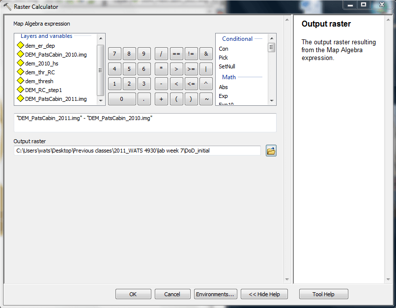
In Raster Calculator subtract DEM_PatsCabin_2010* from* DEM_PatsCabin_2011
Evaluate your results. What are the range of values for this output raster?
What are the units on these values?
Does the range seem reasonable? Apply the color ramp (properties > symbology) “Cold to Hot, Diverging” to this initial DoD. Does the pattern make sense?
Remove uncertain elevation change values
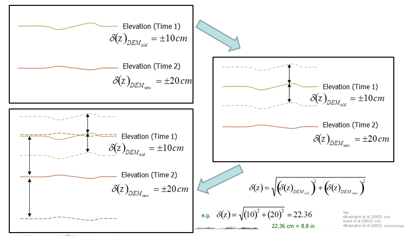
Figure 1. Uncertainty associated with each elevation raster. In our case, we are assuming a 20cm span of uncertainty (+/-10cm).
So if we change this threshold, how does it affect our results? Figure 2 shows a series of DoD outputs with varying levels of uncertainty removed. The image on the left is the raw output. The raster contains all values of elevation change. The image on the right has the largest threshold for uncertainty. (The grey values near 0 m have been removed and an underlying hillshade layer can be seen beneath the red and blue cells showing higher levels of erosion and deposition.)
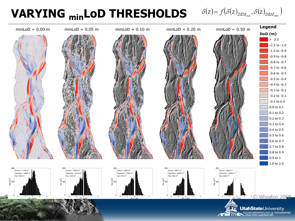
Figure 2. Varying levels of detection (LoD) in uncertainty analysis.
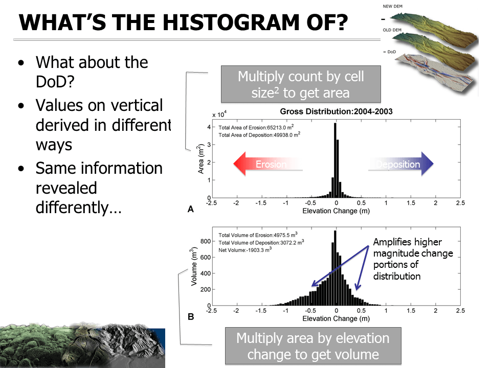
Figure 3. Brief explanation of the threshold histograms (seen in Figure 2) and how they are created.
The actual process of thresholding the DoD looks something like this:
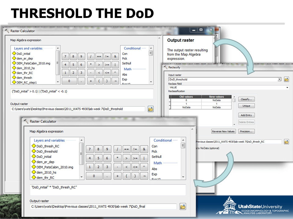
The first step is to reclassify the cell values of the initial DoD to create a binary output raster where cell values of 1 equal areas of certain elevation change (greater than 20cm change), and 0 values being areas of uncertainelevation change (-20cm to 20cm).
In the Reclassify tool window, add your initial DoD and press the Classify… button to open the Classification window:
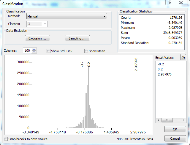
Change the number of classes to 3. If the window is greyed out, temporarily change the classification method to equal interval (ArcGIS glitch). In the Break Values section, change the breaks as shown above (you are setting the 2 breaks and leaving the max value alone). Click OK to return to the Reclassify window.
Assign new values to your classes
In the New values column, reassign the value “1” to all “true” cells (cells with certain elevation change) and assign NoData to the class of uncertain elevation change as shown below.
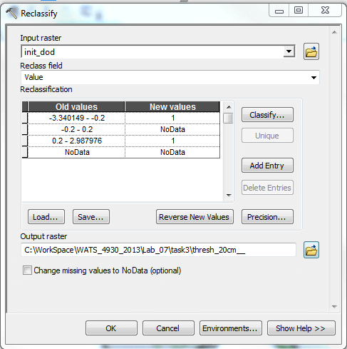
Set your output location and OK to run the reclassify. This output will essentially be used as a mask, as you will see in the next step.
The second step is to multiply your original (initial) DoD with the newly reclassified raster (values of 1 and NoData). This will create an output raster that preserves DoD elevation changes we are highly certain about and removes all elevation changes that are uncertain. If you multiply a cell value by NoData the output is NoData. Therefore the only elevation values that will be output will be in the areas we are certain about.
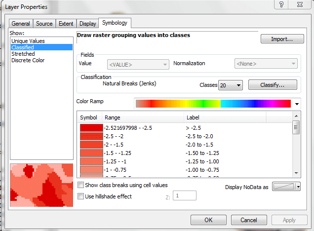
Symbolize your data effectively
You are ready to symbolize your data in a meaningful way. In the final DoD raster’s properties, go to the symbology tab and click to Show: “Classified” values on the left (see below). The symbology you want to import is classified, so you have to take this step for the import to work. Click the Import button and navigate to the Dod_classed_2.5.lyr you downloaded earlier.
Evaluate your results
Evaluate your results taking into consideration the following information about the site: The reach has 13 beaver dams and/or support structures installed. After 2011 high flows, most of the top of reach ponds filled in completely with sediment. There was avulsion in the middle reach where significant downcut occurred as a result of the blowout of one of the major dams. The lower reach ponds aggraded substantially.
If you are confident in your results, create a map illustrating the change in the channel from 2010 to 2011. You have full creative license to display this data in the most effective and convincing way.