gis
Introduction
We have a watershed boundary for the Big Cottonwood Creek watershed (from Lab 6). From Task 1, you know how to derive this watershed from the DEM and from Task 2 you now know something about the structure of the stream network within that watershed. Now we want to analyze the DEM surface to better understand landscape characteristics that might tell us something about the hydrologic and/or geomorphic processes in the watershed. This will be potentially helpful in prioritizing watershed stewardship activities.
Slope Analysis
From ESRI’s GIS dictionary:
The incline, or steepness, of a surface. Slope can be measured in degrees from horizontal (0–90), or percent slope (which is the rise divided by the run, multiplied by 100). A slope of 45 degrees equals 100 percent slope. As slope angle approaches vertical (90 degrees), the percent slope approaches infinity. The slope of a TIN face is the steepest downhill slope of a plane defined by the face. The slope for a cell in a raster is the steepest slope of a plane defined by the cell and its eight surrounding neighbors.
An Example of Curvature
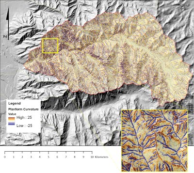
Example of Planform Curvature Calculation
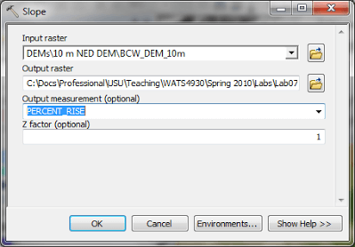
Search for the Slope tool (Spatial Analyst or 3D Analyst), input your filled DEM, name the output something meaningful, change the option for ‘output measurement’ to percent rise (but notice that degrees are an option). Does your output raster make sense? What is the value range and what are the units?

Curvature Analysis
Curvature is a tool we can run to give us more information about the surface slope. For any given cell, we now have a slope measurement. But is that slope shape convex or concave? Would water flow across the cell surface be divergent or convergent? Would it accelerate as it passes over the cell or decelerate? Technically, curvature is a second derivative of the surface, or the rate of change of the slope. And it is proving to be a very effective tool for identifying critical areas on a landscape.
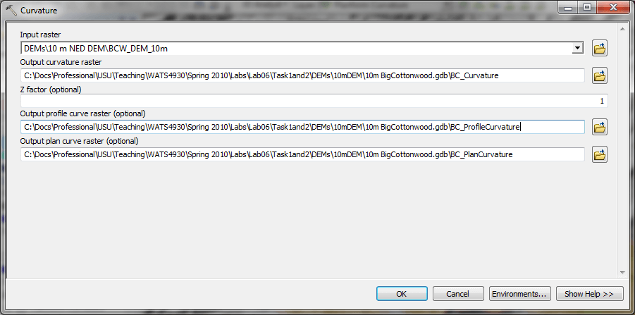
The Curvature tool is found in both the 3D Analyst toolbox and the Spatial Analyst toolbox. Input the pit-filled DEM (from earlier tasks) as your input, and name your output rasters meaningfully. You have the option to (and should) create 2 optional curvature rasters, profile and planform, in addition to the standard curvature output raster.
We highly recommend that you read the information on curvature found at the Curvature Link. Take a close look at your curvature rasters. If you created a stream network raster for Task 2, overlay it. Do you see evidence in the curvature rasters that support where your streams are initiated?
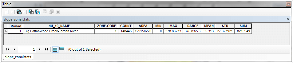
Zonal Statistics
Now we have rasters that represent the slope value and curvature values for every 10m grid cell. How can this information be summarized and translated into something specific to our watershed. For example, what is the average slope value for our watershed, how about the maximum slope?
Zonal statistics provide some tools that allow us to summarize statistics (based on a raster that provides the values) for an area defined by a feature class.
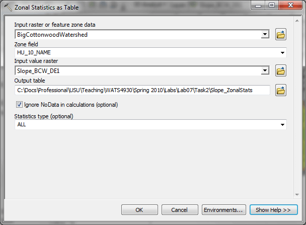
Search for Zonal Statistics and open the Zonal Statistics as Table tool. You will run this tool on your slope, planform curvature, and profile curvature rasters. Use the help window to populate the tool options appropriately (see images below).
You should think about how you might use this information to help summarize your morphometric analyses (i.e. slope and curvature).
Note: inputs will be different for your files.
The Zonal Statistics results are output to a statistics summary table.
-
A table containing summary statistics (minimum, maximum, mean, and standard deviation) for Big Cottonwood Creek watershed slope, planform curvature, and profile curvature
-
- make sure your headers are edited and meaningful and that your numbers are consistently formatted to a level of accuracy your input data can support
-
3 captioned figures of your raster outputs within Big Cottonwood Creek watershed (Optional)
-
- Slope raster
- Profile curvature raster
- Planform curvature raster
See What to Submit section on main Lab 8 page and Lab 8 Rubric (Canvas) for details.