gis

Introduction to Lab

Background

One of the many powers of GIS is combining various data based on spatial location. Information can be obtained from aerial imagery or scanned maps, but to correctly overlay other layers of data, spatial reference or a coordinate system must be defined for, and assigned to, the aerial imagery or scanned maps. This is the process of georeferencing: aligning some type of raster imagery to a map coordinate system. This workshop works through two exercises on georeferencing raster imagery, intended to reinforce some of the coordinate system and projection principles we cover in week 2, as an example from which to build good maps from existing data.

In the second part of this workshop you will be collecting your own data. You will set ground control with a total station and acquire your own aerial imagery by flying a low-altitude blimp. Aerial imagery can be acquired from satellites, fixed-wing aircraft, helicopters, drones, or tethered blimps and balloons. You will then build some georeferenced, high-resolution imagery of the Quad.

Warning: We will be at the mercy of the weather for this lab. Dress accordingly.

Lab Objectives

The two primary objectives of this lab are to 1) teach you how to georeference rasters and 2) reiterate building persuasive and convincing maps.

During this workshop you will learn how to take digital images or maps that are not georeferenced and georeference (or register) them onto an appropriate coordinate system. You will also be exposed to the field data collection process and you see how raw vector and raster data can be collected in the field and then used to produce georeferenced photos. In this workshop exercise you will:

1. Georeference a scanned historical aerial photo to allow you to overlay it on a map
2. Fly a blimp to acquire un-georeferenced, semi-oblique aerial photography
3. Use a total station to acquire ground control points visible in your photo for use in accurately georeferencing the imagery you acquire
4. Georeference a digital aerial photo collected from a small blimp using control points.

Meets Course Learning Outcomes 2, 4 & 5.

Instructions & Lab Tasks

This week, you are working for

USU Facilities Planning

and they have given you somewhat vague instructions to provide them with color, georeferenced aerial photography of the entire quad in UTM (metric) coordinates. The quad is bound on the north, east and west by sidewalks and to the south by a road. Therefore the minimum boundaries (i.e. spatial extent of your work) should include these boundaries. Campus Planning would like you to provide clearly labeled figures illustrating the various products you derive and provide notes on the methods used to derived the maps, the relative quality of the georectification, and the resolution of the imagery shown. They are particularly curious whether or not you can provide them with higher resolution photography then the 2006 HROs from the Utah GIS Portal.

The tasks for this lab can be summarized as follows:

1. Learn the process of georeferencing using an example from St. Helena CA, and produce a figure showing a correctly georeferenced historical aerial photo from 1953 side-by-side with a provided 2002 aerial photograph.
2. Use the data you collect in the field to produce a georeferenced aerial image covering the entire quad using the 2006 HRO 1-foot resolution aerial imagery to perform the georectification.
3. Produce a georeferenced aerial image covering the entire quad using the ground control targets you acquired to perform the georectification.

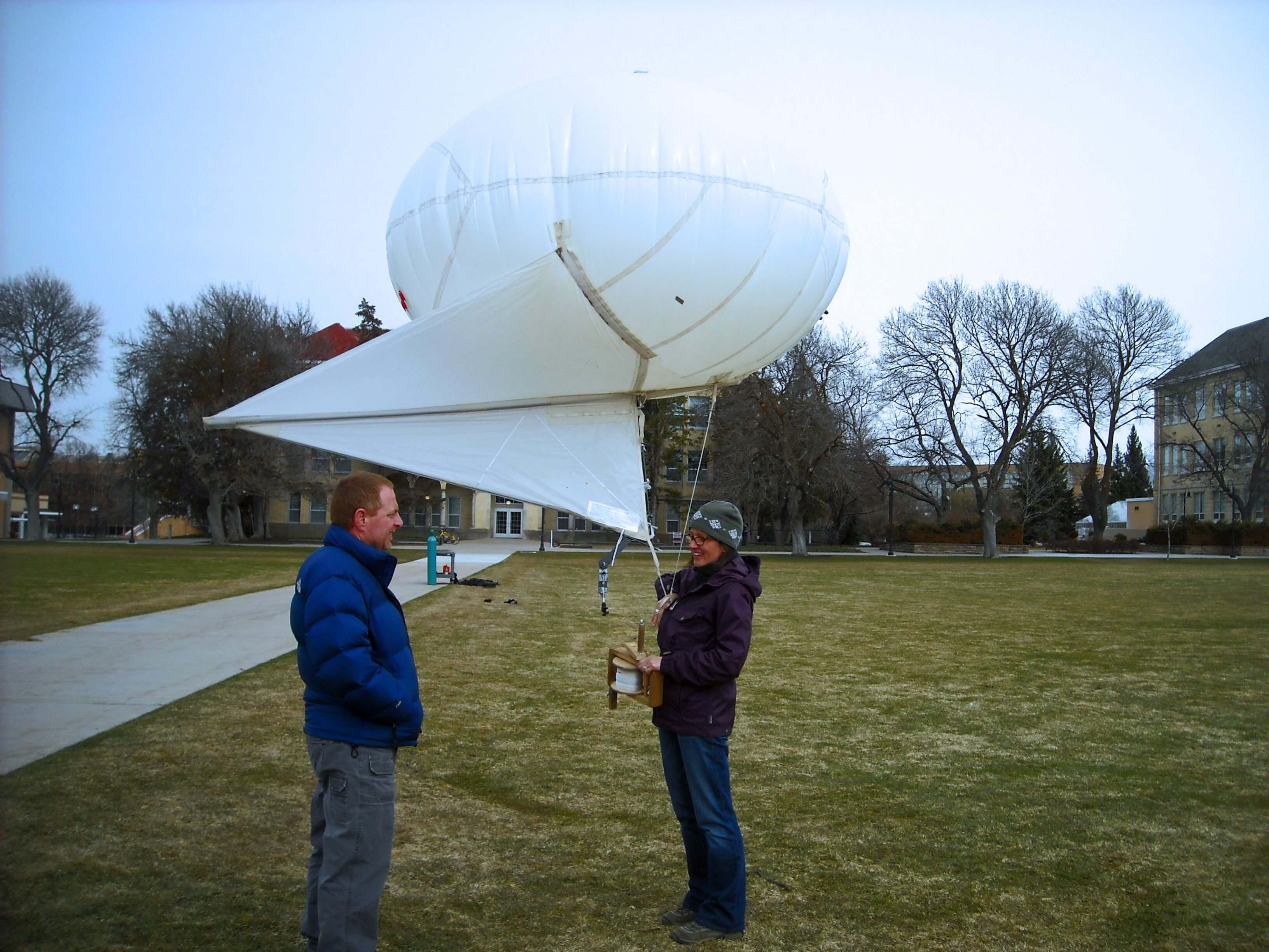
The blimp you will fly over the quad in this lab.

Data for Lab

You are provided with the following new data (inGeoreferencing_StHelena.zip):

• For Task 1, you are provided with a correctly georeferenced aerial photograph from 2002 (2002_SulphurCreek_AP.tif).
• For Task 1, you are provided with a non-georeferenced scanned historical aerial photograph of roughly the same area (1953_StHelena_AP.jpg).
• For Tasks 2 & 3, you will use the data you collected in small groups during lab and secondary data you download yourself. For the secondary data, we recommend the High Resolution Orthophotos available from the AGRC.

Blimp & Old Main

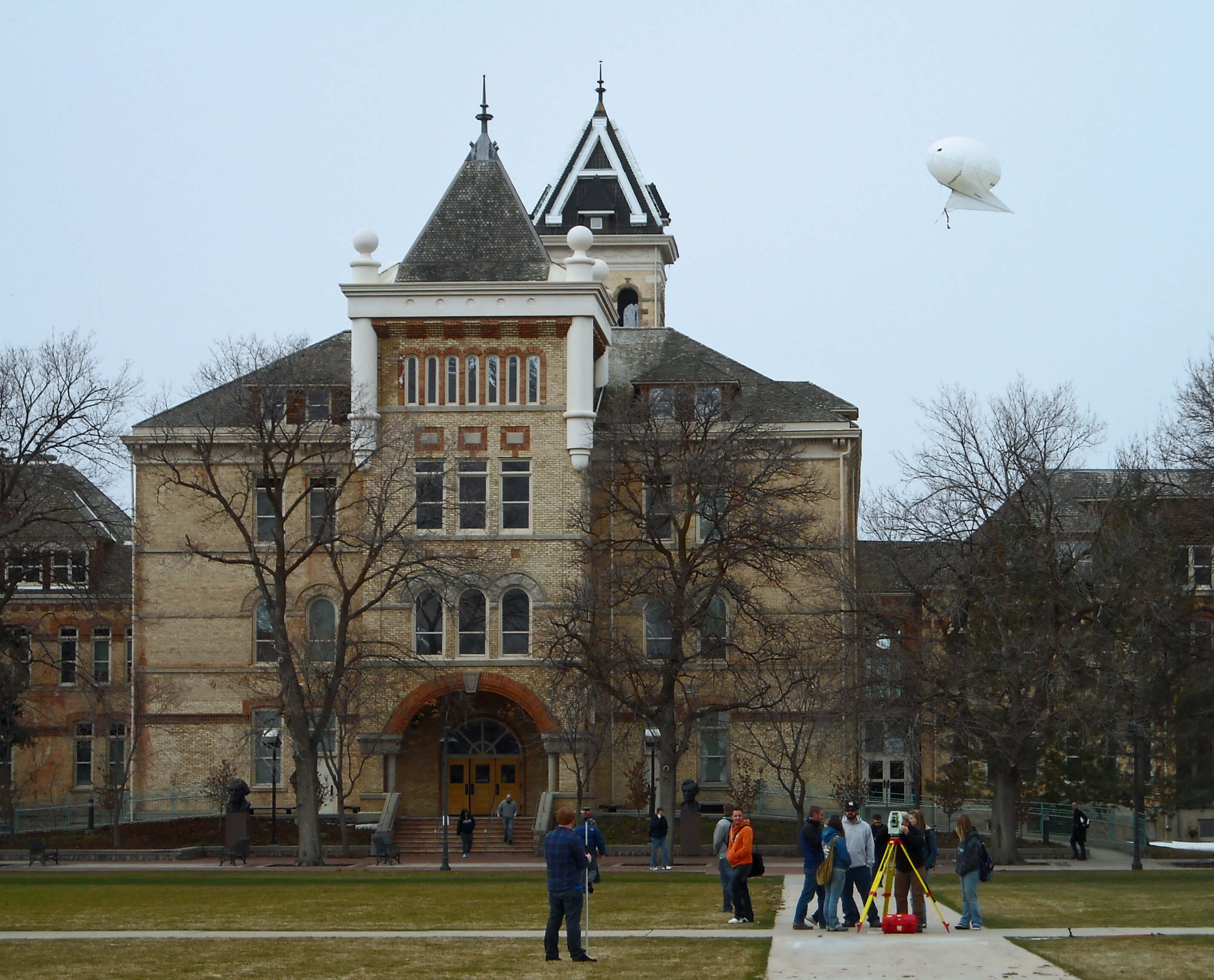
Blimp being flown over quad. Total station in foreground to acquire ground control.

Either TIFFs or JPGs will work, but JPGs come in a zip file with everything you need, whereas you need to manually get the world file and XML auxillary files with the TIFF). You need to figure out what image(s) to download that provide coverage of your survey area (the USU Quad we surveyed). Be sure to report the resolution of the data you choose to download.

The primary source of data for Tasks 2 & 3, is the data you collect in the field. We will make this data available to you by the end of this week. This data consists of 1) aerial photos you collected with the blimp, and 2) coordinate data for the control points you collected with the total station. Here, we tell you where you can retrieve that data. In later sections of these instructions, you will be provided with information to help you decide what subset of the available data you need to download. You are welcome to download it all but you certainly do not need it all! You should only download a subset of the data that your group acquired.

Raw Ungeoreferenced Aerial Imagery

See BlimpSlides_2009.pdf for some examples of georeferenced images from earlier Blimp flights.

Data files from 2014:

Tuesday was a decent day, but camera issues limited the number of images that were captured.
Zip files include photos and CSV file containing target coordinates.

• Tuesday Imagery - Flight A_March 4_2014 52 MB
• Tuesday Imagery - Flight B_March 4_2014 203 MB

There are 19 photos from the first Tuesday flight. The second flight captured 73 photos (Flight B). Each zip file contains a CSV file with the surveyed target coordinates.

The Thursday flights were scrubbed due to high winds.

It took 9 people to bring the blimp down after a harrowing 20 minute flight (fight) by Logan E and others. The Blimp tried so hard to fly off to Idaho it nearly broke the wooden handle, pulling the nails out of the tether reel.

Friday, however, was a great day to fly a blimp. 4 sets of photos were acquired:

• Friday Imagery - Flight A_March 7_2014 94 MB
• Friday Imagery - Flight B_March 7_2014 237 MB
• Friday Imagery - Flight C_March 7_2014 126 MB
• Friday Imagery - Flight D_March 7_2014 138 MB

Again, each Zip file includes photos and a CSV file containing target coordinates.

Flight B recruited some random passers-by to send a special message (see images 5000 to 5006). While the whole quad wasn’t captured, there are some great images here.

Flight D got some great images of the whole quad (Brian R got the blimp up to 250 m!).

Data files from 2013:

• Tuesday Imagery - Flight 1_March 19_2013 Set 1 (includes CSV file and map of targets) 200MB
• Tuesday Imagery - Flight1_March19_2013 Set 2 240 MB

There are approximately 180 photos from the first Tuesday flight. They have been zipped into 2 folders (Set 1 and Set 2) in an effort to make downloading a bit easier. The first folder (Set 1) also contains the CSV file with the surveyed coordinates for each pad. You will want to browse the images and choose one that shows enough pads and overall detail. The remaining Tuesday and Friday flights were scrubbed due to camera malfunction.

Data Files from 2012:

• Thursday 2012 Imagery - Flight 1_north_March22_2012 (Heads up: 500 MB Zip file)
• Thursday 2012 Imagery - Flight 2_south_March22_2012 (Heads up: 550 MB Zip file)

The aerial photos collected with the blimp on Tuesday are not included as winds prevented us from getting enough altitude to capture the entire quad in one image.

Data Files from 2011: (FOR REFERENCE ONLY)

• Tuesday 2011 Imagery (Warning: 2 GB Zip file)
• Thursday 2011 Imagery (Warning: 1.8 GB Zip file)
• Friday 2011 Imagery (Warning: 0.8 GB Zip file)

It’s important to note that changing conditions can greatly affect the ability to collect data with the Blimp. Flights in 2011 were not under ideal circumstances. Tuesday’s lab had decent conditions but the camera settings were off and the images are largely over-exposed and they did not fly high enough to cover the entire quad in one image. Thursday’s flight was better, but the winds were strong. The high altitude images don’t provide a complete coverage of the Quad (in one image) and a strong northwest shifted the coverage outside the quad. The winds were so strong on Friday that the first group could not fly.

Ground Control Data

The coordinate data for the control points (aerial targets) are:

• 2012 Thursday GPS data* - Use this only for Extra Credit*
• 2012 Thursday TS data - Use this one for Task 2

Data Files from 2011: (FOR REFERENCE ONLY)

• TuesdayMarch152011.csv XY coordinate spreadsheet for Tuesday’s (3/15) data collection.
• ThursdayMarch172011.csv XY coordinate spreadsheet for Thursday’s (3/17) data collection.
• FridaydayMarch182011.csv XY coordinate spreadsheet for Thursday’s (3/18) data collection.

Task 1 - Georeferencing a Scanned Historical Image

You need to georeference a scanned historical image (

1953_StHelena_AP.jpg

) based on establishing control points in a more recent (

2002_SulphurCreek_AP.tif

) correctly georeferenced image. This means that the new georeferenced image you produce will take on the coordinate system and projection of the more recent image. You should also assess how good a job you did at georeferencing the imagery, and create a map that convinces your boss that you did the georeferencing correctly.

Produce a figure for your webpage of the correctly georeferenced 1953 St. Helena image. The figure should minimally have two identically sized data frames (preferably with UTM grids), one showing the correctly georeferenced 1953 image, and the second showing the 2002 HRO. Data frames should show the same extents, at the same scales to make an effective comparison. Accompanying your figure you must provide text describing:

• • data source(s),
  • acquisition methods,
  • estimated errors (total RMS),
  • resolution of images,
  • coordinate system information,
  • and any other information that helps convince your audience the georeferencing was done correctly.

• Detailed instructions for Task 1

• Task 2 - Georeference Quad photo using existing imagery

• For task 2, you could define your workflow as follows:

• 1. Download the correctly georeferenced 2006 HRO (high resolution orthophotograph) of the quad (instructions above). Load this image into a new empty ArcMap map document. Ensure the data frame assumes the ‘correct’ coordinate system from this image.
  2. Browse the 100 to 400 images in Picassa that your group acquired during its flight and choose the single best image that provides complete coverage of the quad. This sounds difficult, but you will be surprised how quickly you can browse through all these and choose one that is in focus, is not oblique, and oriented best to suit your needs. If, your group did not fly high enough to have complete coverage of the quad, choose the photo that is the closest to providing complete coverage. For extra credit, you can also browse the other albums and borrow the best image with complete coverage of the quad you can find. To receive extra credit, you will need to produce landscape 11” x 17” PDF with two side-by-side data frames: one showing the georeferenced image from your group and a second showing the georeferenced image you borrowed.
  3. Georeference your image to the UTM coordinate system defined in the 2006 HRO, using points visible in both images as control points. Recall skills learned in Task 1 to complete this part of the lab. Especially, make note of your total RMS and remember to ‘rectify’ your georeferenced images and add it to your map document (remove the unrectified image).
  4. Produce a figure for your webpage of the correctly georeferenced Quad blimp image. The figure should minimally have two identically sized data frames (preferably with UTM grids), one showing your correctly georeferenced blimp image, and the second showing the 2006 HRO. Data frames should show the same extents, at the same scales to make an effective comparison. Accompanying your figure you must provide text describing:
• • • data source(s),
    • acquisition methods,
    • estimated errors (total RMS),
    • resolution of images,
    • coordinate system information,
    • and any other information that helps convince your audience the georeferencing was done correctly.

• ask 3 - Georeference Quad image using Total Station Ground Control

• For task 3, a potential workflow is as follows:

• 1. Start a new empty map document. This map’s data frame should not have a coordinate system associated with it.
  2. Use an ungeoreferenced blimp image (you can use the same one you used in task 2, or select a new one). Add it to your map document.
  3. Add the CSV file to your Arc project and open it to view the contents or open it independently (in Excel, for example).
  4. The layout of the targets will differ depending on how we laid out the pads on any given day, but here is a sample from a previous year:

• 

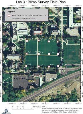
• 1. Georectify the blimp image using your control points and coordinates from the CSV (left click on the pad center, then right-click > add x-y data).
  2. Produce a figure for display on your website. The figure should show your correctly georeferenced blimp image and the surveyed georeferenced targets. Along with your figure, provide text describing:
• • • data source(s),
    • acquisition methods,
    • estimated errors (total RMS),
    • resolution of images,
    • initial and final coordinate systems,
    • and any other information that helps convince your audience the georeferencing and transformation were done correctly.

What to Submit

• Task 1: present the results of your georeferencing in a manner that convinces your audience that the georeferencing was done correctly. At a minimum you should show two identically sized data frames (preferably with matching measured grids), one showing your correctly georeferenced 1953 image, and the second showing the 2002 image. Data frames should show the same extents, at the same scales to make an effective comparison. Accompanying your figure you must provide text describing:
  • data source(s),
  • acquisition methods,
  • estimated errors (total RMS),
  • resolution of images,
  • coordinate system information to inform measured grid,
  • and any other information that helps convince your audience the georeferencing was done correctly.
• Task 2 - Produce a figure for your webpage of the correctly georeferenced Quad blimp image. The figure should minimally have two identically sized data frames (preferably with measured grids), one showing your correctly georeferenced blimp image, and the second showing the 2006 HRO. Data frames should show the same extents, at the same scales to make an effective comparison. Accompanying your figure you must provide text describing:
• • • data source(s),
    • acquisition methods,
    • estimated errors (total RMS),
    • resolution of both images,
    • coordinate system information to inform measured grid,
    • and any other information that helps convince your audience the georeferencing was done correctly.
• Task 3 - Produce a figure for display on your website. The figure should show your correctly georeferenced blimp image and the surveyed georeferenced targets. Along with your figure, provide text describing:
• • • data source(s),
    • acquisition methods,
    • estimated errors (total RMS),
    • resolution of images,
    • initial and final coordinate systems,
    • and any other information that helps convince your audience the georeferencing and transformation were done correctly.
• Decide what is the most effective way to layout your results with a combination of images for your figures and enough contextual text to explain what was asked of you (i.e. introduction and purpose), how you addressed it (i.e. methods), what you produced (i.e. results) and your analysis/interpretation of how well this worked (i.e. discussion).

Make sure your lab conforms to the general lab submission guidelines. Submit a URL for this lab’s webpage.

Additional Resources

Lab Introduction Slides

Lab 10 Slides - Shannon wing Belmont Spring 2013

Tutorial or Step-by-Step Instructions for Specific Tasks

• Fundamentals for Georeferencing a Raster Dataset - From ArcGIS 10 Help
• Georeferencing a Raster Dataset - From ArcGIS 10 Help
• Entering Specific X,Y Coordinates when Georeferencing - From ArcGIS 10 Help. This is what you need to do for Task 2

Web Links:

• Low Altitude Blimps (Poor Man’s Aerial Photography) - From Joe Wheaton’s website
• Aggie Air Flying Circus - Drones from our very own USU Water Lab

This weeks lab is based in the Sulphur Creek Watershed of Northern California, Napa Valley. Form more information, see:

• Grossinger R, Striplen C, Brewster E and McKee L. 2003. Ecological, Geomorphic, and Land Use History of Sulphur Creek Watershed: A component of the watershed management plan for the Sulphur Creek watershed, Napa County, California. A Technical Report of the Regional Watershed Program, San Francisco Estuary Institute, Oakland, CA, 51 pp.
• Watershed Information Center & Conservancy of Napa County

Subpages (1): Task 1: Georeferencing a Scanned Historical Image